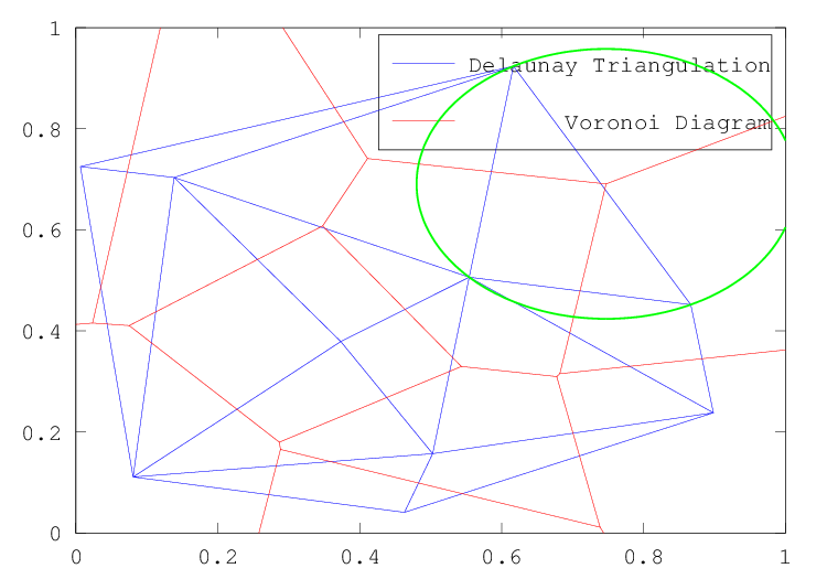
Figure 30.3: Delaunay triangulation and Voronoi diagram of a random set of points
Next: Convex Hull, Previous: Delaunay Triangulation, Up: Geometry [Contents][Index]
A Voronoi diagram or Voronoi tessellation of a set of points s in
an N-dimensional space, is the tessellation of the N-dimensional space
such that all points in v(p), a partitions of the
tessellation where p is a member of s, are closer to p
than any other point in s. The Voronoi diagram is related to the
Delaunay triangulation of a set of points, in that the vertexes of the
Voronoi tessellation are the centers of the circum-circles of the
simplices of the Delaunay tessellation.
Plot the Voronoi diagram of points (x, y).
The Voronoi facets with points at infinity are not drawn.
The options argument, which must be a string or cell array of strings, contains options passed to the underlying qhull command. See the documentation for the Qhull library for details http://www.qhull.org/html/qh-quick.htm#options.
If "linespec" is given it is used to set the color and line style of
the plot.
If an axis graphics handle hax is supplied then the Voronoi diagram is drawn on the specified axis rather than in a new figure.
If a single output argument is requested then the Voronoi diagram will be plotted and a graphics handle h to the plot is returned.
[vx, vy] = voronoi (…) returns the Voronoi vertices instead of plotting the diagram.
x = rand (10, 1);
y = rand (size (x));
h = convhull (x, y);
[vx, vy] = voronoi (x, y);
plot (vx, vy, "-b", x, y, "o", x(h), y(h), "-g");
legend ("", "points", "hull");
Compute N-dimensional Voronoi facets.
The input matrix pts of size [n, dim] contains n points in a space of dimension dim.
C contains the points of the Voronoi facets. The list F contains, for each facet, the indices of the Voronoi points.
An optional second argument, which must be a string or cell array of strings, contains options passed to the underlying qhull command. See the documentation for the Qhull library for details http://www.qhull.org/html/qh-quick.htm#options.
The default options depend on the dimension of the input:
{"Qbb"}
{"Qbb", "Qx"}
If options is not present or [] then the default arguments are
used. Otherwise, options replaces the default argument list.
To append user options to the defaults it is necessary to repeat the
default arguments in options. Use a null string to pass no arguments.
An example of the use of voronoi is
rand ("state",9);
x = rand (10,1);
y = rand (10,1);
tri = delaunay (x, y);
[vx, vy] = voronoi (x, y, tri);
triplot (tri, x, y, "b");
hold on;
plot (vx, vy, "r");
The result of which can be seen in Figure 30.3. Note that the circum-circle of one of the triangles has been added to this figure, to make the relationship between the Delaunay tessellation and the Voronoi diagram clearer.
Additional information about the size of the facets of a Voronoi
diagram, and which points of a set of points is in a polygon can be had
with the polyarea and inpolygon functions respectively.
Determine area of a polygon by triangle method.
The variables x and y define the vertex pairs, and must therefore have the same shape. They can be either vectors or arrays. If they are arrays then the columns of x and y are treated separately and an area returned for each.
If the optional dim argument is given, then polyarea works
along this dimension of the arrays x and y.
An example of the use of polyarea might be
rand ("state", 2);
x = rand (10, 1);
y = rand (10, 1);
[c, f] = voronoin ([x, y]);
af = zeros (size (f));
for i = 1 : length (f)
  af(i) = polyarea (c (f {i, :}, 1), c (f {i, :}, 2));
endfor
Facets of the Voronoi diagram with a vertex at infinity have infinity
area. A simplified version of polyarea for rectangles is
available with rectint
Compute area or volume of intersection of rectangles or N-D boxes.
Compute the area of intersection of rectangles in a and rectangles in b. N-dimensional boxes are supported in which case the volume, or hypervolume is computed according to the number of dimensions.
2-dimensional rectangles are defined as [xpos ypos width height]
where xpos and ypos are the position of the bottom left corner. Higher
dimensions are supported where the coordinates for the minimum value of each
dimension follow the length of the box in that dimension, e.g.,
[xpos ypos zpos kpos … width height depth k_length …].
Each row of a and b define a rectangle, and if both define multiple rectangles, then the output, area, is a matrix where the i-th row corresponds to the i-th row of a and the j-th column corresponds to the j-th row of b.
See also: polyarea.
For a polygon defined by vertex points (xv, yv), return
true if the points (x, y) are inside (or on the boundary)
of the polygon; Otherwise, return false.
The input variables x and y, must have the same dimension.
The optional output on returns true if the points are exactly on the polygon edge, and false otherwise.
See also: delaunay.
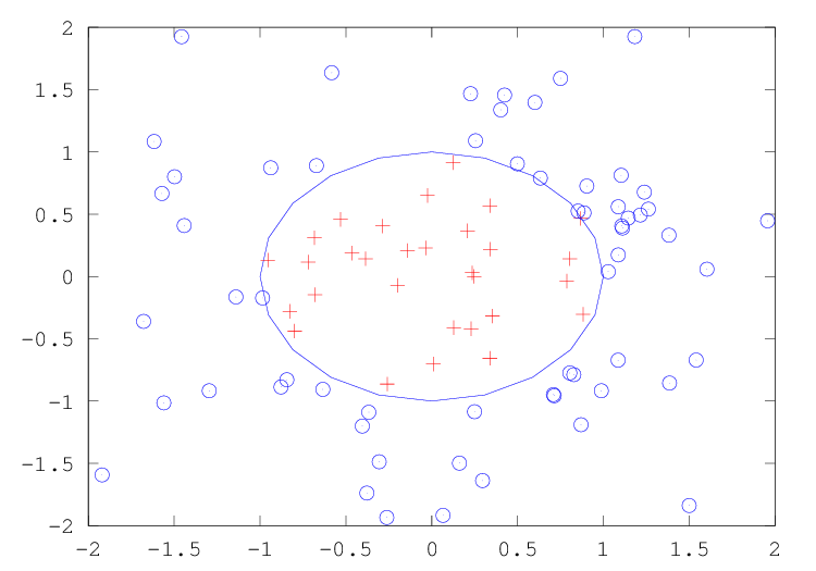
An example of the use of inpolygon might be
randn ("state", 2);
x = randn (100, 1);
y = randn (100, 1);
vx = cos (pi * [-1 : 0.1: 1]);
vy = sin (pi * [-1 : 0.1 : 1]);
in = inpolygon (x, y, vx, vy);
plot (vx, vy, x(in), y(in), "r+", x(!in), y(!in), "bo");
axis ([-2, 2, -2, 2]);
The result of which can be seen in Figure 30.4.
Next: Convex Hull, Previous: Delaunay Triangulation, Up: Geometry [Contents][Index]